By V. Réville, A.P. Rouillard, N. Poirier, R. Pinto & M. Indurain
ARTICLES DESCRIBING SOMES FEATURES OF THE TOOL
Rouillard et al, 2020, Models and Data Analysis Tools for the Solar Orbiter mission, Astronomy and Astrophysics, A&A 642, A2 (2020) (https://www.aanda.org/articles/aa/pdf/2020/10/aa35305-19.pdf)
Poirier et al. 2021, Exploiting white-light observations to improve estimates of magnetic connectivity, Frontiers in Space Physics, Frontiers in Astronomy and Space Sciences, Volume 8, id.84 (2021) (https://www.frontiersin.org/articles/10.3389/fspas.2021.684734/full)
GENERAL INFORMATIONS
The Magnetic Connectivity Tool can help you estimate the solar source location of the solar wind and energetic particles measured by different spacecraft. In doing so, the tool will model the coronal and interplanetary magnetic field based on different assumptions and techniques. Currently the coronal model is primarily based on a magnetostatic reconstruction technique called the Potential Field Source Surface (PFSS) model and the interplanetary magnetic field is assumed to be a Parker spiral. This is schematised in the following diagram.
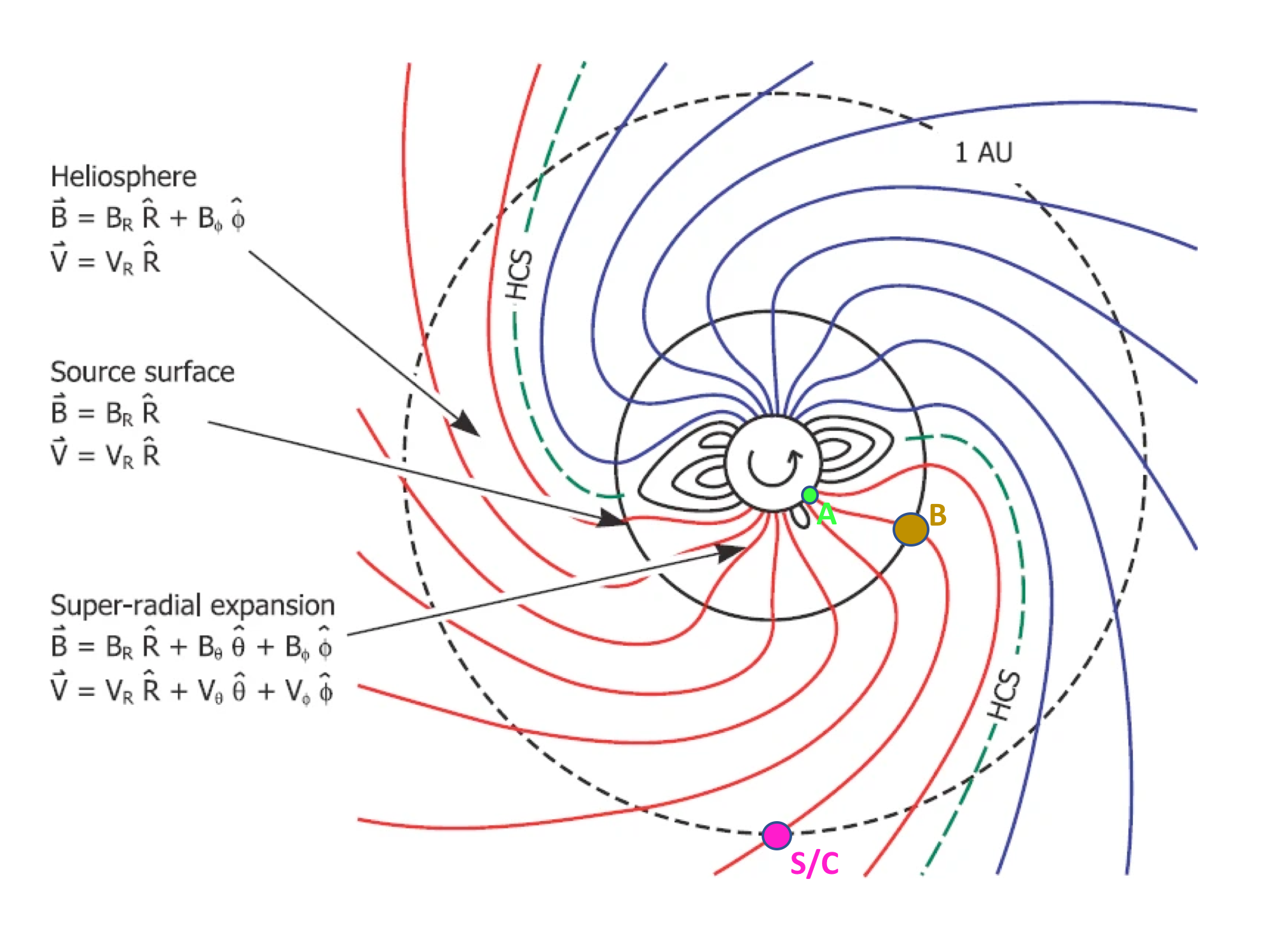
There are two possible directions of propagation, either from the Sun to a S/C or from a S/C to the Sun.
A first critical parameter to define magnetic connectivity will be the speed of the solar wind at the spacecraft because this speed will define the shape of the Parker spiral considered in the tracing. This spiral will define the longitudinal difference between the spacecraft of interest (S/C) and point B at the outer boundary of the coronal model (Schematic 1). Once point B is determined by the tool, the latter knows which field line to trace from B to the solar surface in the coronal model. When solar wind speed measurements are available (public data), the tool uses those specific measurements to compute the shape of the spiral (the speed is then displayed in the legend of the Carrington map as ‘FP measured SW’ and give you the speed considered). For Solar Orbiter the tool will either use the scientific fully calibrated data from the Proton Alpha Sensor or if the data is not yet available it will retrieve the Low Latency Data from PAS released by the Solar Orbiter archive. So information about the solar wind speed is obtained in quasi real time.
When solar wind speed data is not available (never obtained or not public) then the tool assumes two possible speeds for the solar wind, either slow (300 km/s) or fast (800 km/s). These two extreme speeds will be used to compute with the corresponding two spirals the two connectivity points B and then trace from these two points (B) down to the solar surface (A) in the coronal model (see the corresponding legend in the Carrington map). In fact the tool does more than that, it will consider a distribution (cloud) of possible points around each point B and trace hundreds of field lines to give you an estimate of the level of uncertainty in the tracing. This is why you see two clouds of coloured points at the solar surface for each spacecraft.
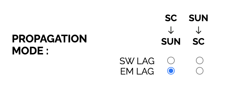
A second critical parameter that must be computed by the tool is the difference between the time a solar wind parcel (or an energetic particle) has been measured by a spacecraft and its release time from the Sun that will in turn define the time of the coronal model to be considered. For example if you decide to start at a spacecraft and go back to the Sun (because you have identified a feature of interest at the spacecraft and want to find its source at the Sun) then the propagation time of that feature from point B to S/C will be calculated by the tool and used to define the date of the magnetogram that should be considered to reconstruct the coronal magnetic field reconstruction. A nearly relativistic particle will have a much shorter propagation time (a few minutes) compared with a solar wind parcel (typically 1-5 days depending on wind speed and the heliocentric distance of the spacecraft). Therefore the tool offers in addition to considering solar wind propagation times (SW lag), the possibility to assume the time of propagation of electromagnetic radiation (EM lag) so that someone who wants to find the source location of very fast solar energetic particles can also use the tool. The EM lag is currently set to zero because the cadence of the data/images shown in the tool is typically of the order of 6 hours compared with EM propagation time of photons from the Sun to the different spacecraft of a few minutes only. Once a lag type (SW lag or EM lag) is chosen the tool will take the spacecraft date/time and calculate the launch date/time at the Sun and consequently identify the magnetogram that should be used to model the coronal magnetic field.
The tool will provide estimates of magnetic connectivity either at the solar surface if you compare say your connectivity with a magnetogram or an EUV image (that capture features located in the corona but very close the solar surface) or higher up in the atmosphere (5 solar radii) if you consider a map of helmet streamers taken by coronagraphs (since 5 solar radii is above the outer boundary of the model, the tool only uses a Parker spiral for tracing and no coronal model is considered).
You can choose from a broad range of maps from the tool as catalogues of identified features (active regions, flares and soon CME sources).
If the date/time falls in the future, the tool uses forecasts of magnetic connectivity provided by the ADAPT project. Forecasts of magnetic connectivity will be useful to Solar Orbiter operations and are provided up to 10 days out in the future. We will show an example in the pdf version.
CAVEAT
Data availability: the Magnetic Connectivity Tool collects data from a wide range of data providers. These data pipelines may be temporarily interrupted for a multitude of possible reasons such as for instance issues with the ground-based and spaceborne observatories making the measurement or interrupted data transfers. As soon as the data transfer is resumed the Magnetic Connectivity Tool repopulates its database with all the available data. Consequently when a feature is not available in the tool, we recommend that you try the tool a day later. If the issue persists please send us a message so we can isolate the issue and act to resolve the problem as quickly as we can.
Limitations of PFSS: the PFSS model used in the Magnetic Connectivity Tool is the simplest approach to model the magnetic field of the solar corona. It has the advantage that it is simple to develop and implement and requires relatively modest computer resources. It assumes that the solar magnetic field is in a potential state and therefore has no electric currents. This potential field assumption should be considered as representative of a ‘minimum energy state’ that the corona tends towards during quiet solar conditions, i.e. when there are no Coronal Mass Ejections or other strong disturbances. PFSS models cannot directly incorporate time-dependent phenomena, such as magnetic reconnection, and do not include plasma or its effects. When the corona is disturbed by strong eruptions, the magnetic representation provided by PFSS and therefore the magnetic connectivity provided by the tool is likely to be highly inaccurate. PFSS also assumes that the magnetic field is radial at a pre-defined spherical ‘source surface’, while this is reasonable during solar minimum conditions, deviations from a spherical source surface are likely to develop during solar maximum periods (Riley et al. 2006). In contrast, Magneto-Hydrodynamic (MHD) simulations account for currents, do not assume a spherical source surface and are capable of capturing time-dependent phenomena. They are considered more accurate however they are much more demanding computationally and usually run at much lower resolution that PFSS and more seldomly. Future updates of the Magnetic Connectivity Tool will include such 3-D MHD simulations for specific dates.
Reference: Riley P., Linker J.~A., Mikic Z., Lionello R., Ledvina S.~A., Luhmann J.~G., 2006, ApJ, 653, 1510. doi:10.1086/508565
Download the full pdf version of this tutorial, with different cases studying.